A single laser scanner approach.

We've been struggling with the problems of building a scanning laser rangefinder that can do all the tasks we need.

To summarize, we need to be able to do all these things:

• Detect non-flat terrain at 50 meters and 40MPH.
• See enough field of view at 50 meters to drive on a more or less straight road.
• Map to a 15cm level of detail at 20-25 meters and 25MPH.
• See enough field of view at 20-25 meters to drive on a curvy road.
• See obstacles and holes as close as the front bumper at speeds from zero to 10MPH.

Here is a single-laser design that meets those criteria.

It's a polygon scanner, much like the one described in Note 12. But instead of having 24 faces, it only has 6, which results in a prism a quarter of the diameter and a sixteenth of the weight. By orienting those six faces appropriately, we can get a scan pattern like this:

Scan pattern of a six-face prism scanner. The furthest line, 50 meters out at maximum speed, is scanned twice, with the two faces with that tilt equally spaced around the prism. The other lines are each scanned once; the order does not matter.

Lincoln Laser builds polygon scanners to order, with pricing around $3700 in quantity 1. We can order any face tilts we want. Acuity can also fabricate such wheels, but Lincoln's primary business is building these devices.

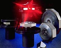Various Lincoln Laser polygon scanner wheels. (From Lincoln Laser ad.)

Design analysis

15cm scan density at 50m range

Assume we want one data point in every 15cm cell at 50m. (The CMU Navlab off-road work used a 15cm scan density.)

The scan circle at 50m is 314m, or 2095 data points spaced 15cm apart.

Assume we hit the longest range circle twice per rev, using a 6-sided prism (thus a 120 degree arc is scanned.)
We need a data point every 15cm of forward movement. 40mph is 59fps, or 18 m/sec, or 120 scan lines/sec.
At once per rev, we would need 120 revs/second to get enough scan lines.
At twice per rev, we would need 60 revs/second to get enough scan lines.
60 * 2095 = 125,700 points/sec.

That point scanning rate is a bit beyond what can be easily achieved.

20cm scan density at 50m range

At a lower scan density, we have this:

Scan circle is 314m or 1570 data points.
At 40mph, we would need 90 scan lines/sec.
At twice per rev, we would need 45 revs/sec. 45*1570 = 70,650 points/sec. Prism speed is 2700 RPM.

At 20 MPH and 25M, we have a scan circle of 157m. We are going slower, so the scan lines are closer together.
Points are now 10cm apart in both dimensions.

Speeding up to 25mph gives a scan line separation of 12.5cm.

These are acceptable numbers.

Driving with a multiline scanner

What does it look like to drive with a scanner like this?

The general idea is that at long ranges and high speeds, we need a reasonably flat road ahead. Thus, at long range, a low-detail model of the terrain is enough, provided that the model is conservative. That is, we don't need to map every rock and pothole; we need only distinguish between "flat" and "non-flat" at a coarse level of detail. At slower speeds, we may have to steer around, or over, obstacles. So we need a terrain model with finer detail at short range.

High speed operation

Best case, we're going along at 40MPH, collecting a scan line every 20cm. So we collect 25 points per square meter at maximum range. That's not bad.

We only go to high speed (40MPH) when the terrain is reasonably good, that is, free of obstacles for a reasonable road width.. At the long range (25-50m) needed for high speed, we thus need only a coarse grid. Suppose we use a 1 meter grid for long range data. We would then get 25 points per cell as we move forward, which is good enough to make a good flatness estimate, and allows the loss of a reasonable number of points due to noise, vibration, etc

The CMU rule was that you needed 5 points to get a height, tilt, and flatness estimate for a cell. So we have enough data to build up a 50cm grid, with about 6 points per cell. But that would assume good registration between scans. Bouncing around at 40MPH, we're probably better off derating the cell size by a factor of 2, which gives us 4x as many points. We can tweak these numbers once we get the system running; the goal here is to see if it can work using conservative assumptions. If we don't get 5 points for a cell on our path, we can't go there.

Suppose we build up certainty grids with 25cm cells out to 12 meter range, 50cm cells out to 25 meter range, and 1m cells out to 50 meter range. We then collect an average of 25 points per 1m cell at 50 meters and 40MPH. This gives us confidence that the road ahead is flat enough to traverse.

Low-speed/short range operation

The finer grids may not be fully updated at high speed. At 40MPH, we only have one scan line every 40cm at 25 meters (remember that the 50m scan arc is scanned twice per rev, but the other ones are only scanned once.) The scan arcs cover half as much ground at 25m, so the density along the arc doubles. So our scanning raster at 25m and 40MPH is 10cm x 40cm. This is enough to update a 1m grid, but too low for a 50cm grid. At 25MPH, the scan arcs are closer together; we get an arc every 25 cm of travel, with 5 points across the arc. This is enough to update a 50cm grid. So we have to slow to 25 if we are not detecting a flat path ahead. That's reasonable.

Similarly, we can update the 25cm grid properly only at speeds below 12MPH or so.

Certainty grids for this scanner 0.25m cells at 0 to 2.5 meter range 0.5m cells at 12.5 to 25 meter range 1m cells at 25 to 50 meter range

Data reduction

Data reduction follows (roughly) the CMU off-road model. For each grid cell for which we have at least 5 data points, we compute an average height, a surface normal, and deviation from the plane determined by the height and the surface normal. This last value is a measure of roughness. Data is collected at the outer arc of each scan area as the vehicle moves forward. As we move forward, our position becomes less certain, so the map is "blurred" as we move.

Two main processing subsystems use these maps. One answers the simple question "Can we go here, and if so, how fast", and the other, a more complex system, does route planning in difficult situations.

Incidentally, we may want to use hexagonal, rather than square grids.

Hills

The analysis so far assumes flat terrain. Now we look at hills.

The scanner needs to tilt up and down, by about 30-50 degrees, to deal with hilly terrain. Maximum downward tilt stops where the scanner almost sees the front bumper. Considerable upward tilt might be useful if we're in a gully.

Tilt is usually controlled by a servoloop that tries to keep the outermost scanning arc at 1.5 to 2 stopping distances.

More to follow.